Back to basics with Pandas

In the spirit of our last post, let’s take things back to basics with a simple end-to-end data analysis example.

Back to basics with pandas, plotnine, and sklearn

In this colab we do a quick review of the ‘data science basics’:

• Download a (small) dataset from an online repository.
• Use pandas to store and manipulate the data.
• Use plotnine to generate plots/visualizations.
• Use scikit-learn to fit a simple logistic regression model.

# @title Imports

import numpy as np
import pandas as pd
import plotnine as gg
import requests
import sklearn

Let there be data

Let’s fetch the famous Iris dataset from the UCI machine learning datasets repository.

# The URL for the raw data in text form.
data_url = 'https://archive.ics.uci.edu/ml/machine-learning-databases/iris/iris.data'

# Column names/metadata.
feature_columns = ['sepal_length', 'sepal_width', 'petal_length', 'petal_width']
target_columns = ['target']

# Fetch the raw data from the website.
response = requests.get(url=data_url)
rows = response.text.split('\n')
data = [r.split(',') for r in rows]

# Turn it into a dataframe and drop any null values.
df = pd.DataFrame(data, columns=feature_columns + target_columns)
df.dropna(inplace=True)

# Fix up the data types: features are numeric, targets are categorical.
df[feature_columns] = df[feature_columns].astype('float')
df[target_column] = df[target_column].astype('category')

Take a quick look at the data

# Look at the raw data to check it looks sensible.
df.head()

	sepal_length	sepal_width	petal_length	petal_width	target
0	5.1	3.5	1.4	0.2	Iris-setosa
1	4.9	3.0	1.4	0.2	Iris-setosa
2	4.7	3.2	1.3	0.2	Iris-setosa
3	4.6	3.1	1.5	0.2	Iris-setosa
4	5.0	3.6	1.4	0.2	Iris-setosa

# Look at some summary statistics.
df.describe()

	sepal_length	sepal_width	petal_length	petal_width
count	150.000000	150.000000	150.000000	150.000000
mean	5.843333	3.054000	3.758667	1.198667
std	0.828066	0.433594	1.764420	0.763161
min	4.300000	2.000000	1.000000	0.100000
25%	5.100000	2.800000	1.600000	0.300000
50%	5.800000	3.000000	4.350000	1.300000
75%	6.400000	3.300000	5.100000	1.800000
max	7.900000	4.400000	6.900000	2.500000

# 6.1 KB ... now that's some #bigdata ;)
df.info()

<class 'pandas.core.frame.DataFrame'>
Int64Index: 150 entries, 0 to 149
Data columns (total 5 columns):
sepal_length    150 non-null float64
sepal_width     150 non-null float64
petal_length    150 non-null float64
petal_width     150 non-null float64
target          150 non-null category
dtypes: category(1), float64(4)
memory usage: 6.1 KB

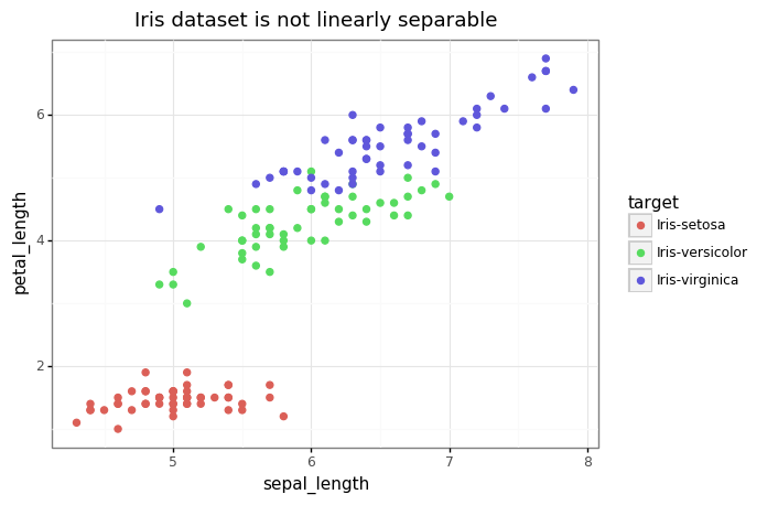
# Let's take a visual look at the data now, projecting down to 2 dimensions.
gg.theme_set(gg.theme_bw())

p = (gg.ggplot(df)
     + gg.aes(x='sepal_length', y='petal_length', color='target')
     + gg.geom_point(size=2)
     + gg.ggtitle('Iris dataset is not linearly separable')
    )
p

Fitting a simple linear model

Let’s get ‘old school’ and fit a simple logistic regression classifier using the raw features.

In the binary case, this is a linear probabilistic model with Bernoulli likelihood given by

\[\mathcal{L}\left(\pmb{x}, y \lvert \pmb{x}\right) = f(\pmb{x})^y (1 - f(\pmb{x}))^{1-y},\]

where \(f(\pmb{x}) = \sigma\left(\pmb{w}^T\pmb{x}\right)\).

Assuming the dataset \(\mathcal{D}=\left\{\pmb{x}^{(i)}, y^{(i)}\right\}_{i=1}^{n}\) is iid, the negative log-likelihood yields the familiar cross-entropy loss:

\[\begin{aligned} \log\mathcal{L}\left(\mathcal{D} \lvert \pmb{w}\right) &= \log\prod_{i=1}^{n} \sigma\left(\pmb{w}^T\pmb{x}^{(i)}\right)^{y^{(i)}} \left(1 - \sigma\left(\pmb{w}^T\pmb{x}^{(i)}\right)\right)^{1-y^{(i)}} \\ &= \sum_{i=1}^n y^{(i)}\log f\left(\pmb{x}^{(i)}\right) + (1-y^{(i)})\log\left(1 - f\left(\pmb{x}^{(i)}\right)\right) \end{aligned}\]

This is a convex and trivially differnetiable objective that we can optimize with gradient-based methods. We’ll defer this to scikit-learn (which also does some other tricks + regularization).

# Create a logistic regression model.
model = sklearn.linear_model.LogisticRegression(solver='lbfgs',
                                                multi_class='multinomial')

# Extract the features and targets as numpy arrays.
X = df[feature_columns].values
y = df[target_column].cat.codes  # Note that we 'code' the categories as integers.

# Fit the model.
model.fit(X, y)

# Compute the model accuracy over the training set (we don't have a test set).
pred_df = df.copy()
pred_df['prediction'] = model.predict(X).astype('int8')
pred_df['correct'] = pred_df.prediction == pred_df.target.cat.codes
accuracy = pred_df.correct.sum() / len(pred_df)
print('Accuracy: {:.3f}'.format(accuracy))

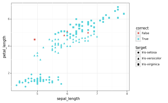
Accuracy: 0.973

# Let's look again at the data, highlighting the examples which we mis-classified.
p = (gg.ggplot(pred_df)
     + gg.aes(x='sepal_length', y='petal_length', shape='target', color='correct')
     + gg.geom_point(size=2)
    )
p